04 Feb Turbulent Dispersion
Revisiting Atmospheric Diffusion at the Cloud-Clear Air Interface
Numerical Simulation cloud-clear air interfaces
Direct numerical simulations (DNS) of a decaying turbulent layer at a cloud top reveal enhanced diffusivity in the mixing region between cloudy and clear air. In this research, we build upon the foundational work of Lewis F. Richardson (1926), who introduced a distance-neighbour distribution function, Q(ℓ, t), to describe the dispersion of particles over a separation distance ℓ in turbulent flows. Due to its definition, the evolution of Q can be modeled by a diffusion-type equation:
∂Q/∂t = ∂/∂ℓ ( F(ℓ, t) ∂Q/∂ℓ )
A central challenge is identifying the correct form of the diffusion function F(ℓ, t). Richardson originally proposed a scaling of the form F(ℓ) ~ ℓ4/3, which laid the foundation for the well-known Richardson–Obukhov law (ℓ2 ~ t3) applicable in homogeneous, isotropic turbulence. This theory has been extensively revisited and refined, including significant contributions by Obukhov and others.
Our work extends this classical framework into a more complex and realistic setting through direct numerical simulations (DNS) of a time-decaying turbulent, shear-free layer. This simulated domain represents a localized segment of a top warm cloud boundary, modeled as a multiphase system involving air, water vapor, and liquid water droplets.
A key focus is the interfacial region between the cloud and surrounding clear air—a highly anisotropic and intermittently turbulent zone. In this region, we anticipate that the diffusion function F should reflect the unique microphysical and turbulent properties at play. Based on our DNS data, we propose two alternative scaling laws for F(ℓ, t), each incorporating relevant thermodynamic and turbulence parameters:
Proposed Scaling Laws
- Scaling Law 1: F(ℓ, t) ~ ε2/3(t) <κs(t)> τp ℓ2/3
- Scaling Law 2: F(ℓ, t) ~ ε2/5(t) <κs(t)> τp1/5 ℓ6/5
Here:
ε(t): turbulent kinetic energy dissipation rate
<κs(t)>: kurtosis of supersaturation fluctuations
τp: phase relaxation time, characterizing droplet response to supersaturationThese scaling models are consistent in order of magnitude with values originally observed by Richardson and reported in historical boundary layer data (e.g., Schmidt 197, Akerblom 1908, Taylor 1914, Hesselberg & Sverdrup 1915).
Observed Parameter Ranges from Simulations
Within the temporal window t/τ0 ∈ [1, 6], the DNS results show:
- Energy dissipation rate: ε(t) ∈ [10, 100] cm²/s³
- Supersaturation kurtosis: <κs(t)> ≈ 3 in the cloud; 15–30 in the mixing region
- Phase relaxation time: τp ≈ 10 in the cloud; 20–80 in the mixing region
Our results demonstrate a significant increase in turbulent diffusivity within the mixing region, aligning well with empirical observations from early atmospheric studies. This highlights the need to incorporate local microphysical variability in turbulence diffusion models, especially in cloud-edge regions where phase changes and thermodynamic fluctuations are prominent.
The figure below show the computed two turbulent diffusion trends and the large diffusion increase in the mixing region.
Figure 1: The transparency level shows the time decay. The interfacial cloud boundary is an instance of anisotropic shear-less turbulence where transport and intermittency are particularly intense
Figure 1. Illustrates the dispersion pf the water droplets with an initial monodispers size distribution (droplet diameter: 15 microns) in a mixing process under stable stratification. The evolution of the dispersion over 25 eddy turnover times can be observed in the accompanying Movie.
Figure 2. illustrates the dispersion of the water droplets with an initial monodispers size distribution (droplet diameter: 15 microns) in a cloud region under stable stratification
Figure 3. Depicts the dispersion of water droplets, initially having a monodisperse size distribution with a droplet diameter of 15 microns, during a mixing process under unstable stratification See Movie
Figure 4. illustrates the dispersion of water droplets with an initial monodisperse size distribution (droplet diameter: 15 microns) in a cloud under unstable stratification see Movie
Figure 5. COLLISION-COALESCENCE of WATER DROPLETS inside atmospheric clouds
The visualization shows a monodisperse population of water droplets within the lower interface region (shaded in gray) of a numerical warm cloud simulation, situated at an altitude of approximately 1000–2000 meters above sea level. Droplets were initially 15 µm in diameter and are enlarged here for better visibility.
Figure 6. Water Droplet Dispersion in a Turbulent Shearless Mixing Layer
Water droplet subsets are initialized at distinct spatial locations within the flow field, and their subsequent dispersion and mixing are tracked over time. This allows for the analysis of how varying initial conditions influence the overall dispersion behavior in a turbulent shearless mixing layer. The visualization illustrates the distribution of droplets for the case of an initially monodisperse distribution.
Figure 6. Water Droplet Dispersion in a Turbulent Shearless Mixing Layer
Water droplet subsets are initialized at distinct spatial locations within the flow field, and their subsequent dispersion and mixing are tracked over time. This allows for the analysis of how varying initial conditions influence the overall dispersion behavior in a turbulent shearless mixing layer. The visualization illustrates the distribution of droplets for the case of an initially Polydisperse distribution.
A novel measurement system developed by the Philofluid research group at Politecnico di Torino employs a cluster of miniaturized radiosondes to monitor atmospheric fluctuations over a 10 km range. This innovative approach extends beyond traditional cloud observation, offering valuable applications in environmental monitoring, particularly in urban and industrial areas.
The current in-field measurement setup includes a network of ground stations and a cluster of miniaturized radiosondes, which were developed as part of the H2020-COMPLETE project.
For further information, please refer to the section dedicated to HOUSEFLIES.
This newly designed and developed system offers three key advantages:
Direct Measurement of Lagrangian Dispersion
Enables direct quantification of Lagrangian turbulent dispersion and diffusion in the field.Monitoring Fluctuations in Warm Clouds (ABL)
Facilitates the tracking of various physical parameter fluctuations within warm clouds.Enhanced Understanding of Cloud Dynamics
Provides simultaneous measurements from multiple cloud locations, offering valuable insights into small- to medium-scale cloud behavior.
Between June 2021 and June 2024, we carried out a series of in-field experiments using both single and multiple radiosondes under diverse environmental conditions. The accuracy of the sensors was thoroughly validated by comparing measurements against reference values from traceable instruments at established meteorological stations, including those operated by INRIM, ARPA-Piemonte, the UK Met Office, OAVdA, and the Chilbolton Observatory.
Comprehensive validation tests—ranging from single-sonde deployments to dual soundings and multiple tethered sondes—are detailed in the section dedicated to HOUSEFLIES. These validation efforts laid the groundwork for free-flying cluster experiments in the atmospheric boundary layers (ABLs) of both Alpine (Valle d’Aosta, Italy) and near-coastal (Chilbolton, UK) environments. These campaigns assessed the feasibility of analyzing atmospheric fluctuations and applying Richardson’s distance-neighbor graph statistics to study turbulent dispersion.
A radiosonde cluster experiment enables detailed observation of atmospheric flow by simultaneously gathering data from multiple regions within the flow domain. By combining the trajectory data of each radiosonde with the corresponding physical measurements recorded along their paths, we can generate a multi-Lagrangian dataset.
This dataset is highly valuable for analyzing turbulent fluctuations and Lagrangian dispersion within the atmospheric boundary layer and warm clouds. Additionally, using clusters to track multiple physical quantities significantly increases the potential for Lagrangian cross-correlation analyses across various parameters.
Validation for the measurement system
The initial field test aimed to evaluate different radiosondes (Ballon-radioprobe) configurations and validate sensor measurements against a fixed point station. These radiorobes were assembled and tested near the Vaisala WXT510 station at the INRIM campus in Turin, Italy, on July 20th, 2021.
Figure 1: The radioprobe electronic board was tested in two different radiosonde configurations. (a) Configuration A: The radioprobe board is outside the balloon. (b) Configuration B: The radioprobe board is in a pocket inside the balloon.
Figure 2: Comparison of radiosonde sensor readings (configurations A & B, refer to Figure 1) for details on configurations. First Column (a, c, e): Sensor readings on the ground (not attached to the balloon). The gray shaded regions highlight readings after the warm-up period for the radiosonde sensors. Note that the continuously operating WXT510 station (reference) does not exhibit a warm-up transient. Second Column(b, d, f): Comparison of sensor readings after attaching the radiosonde to the balloon.
Figure 3. Velocity measurements of the radioprobe during the dual-sounding experiment on June 9, 2021, at Levaldigi Airport, Cuneo, Italy. (a) 3D wind speed components and magnitude derived from GNSS. (b) Comparison of horizontal wind speed with RS41-SG probe (raw and resampled data for COMPLETE radioprobe shown). (c) Power spectrum comparison of wind speed fluctuations (Nyquist frequency reference lines included), denoted as fs/2 = 0.125s−1. Alongside the raw spectrum dataset, two trend lines (in yellow and violet) are presented for reference.
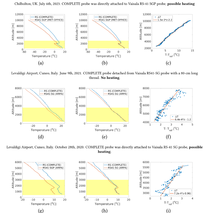
Figure 4: Comparison of temperature measurements from the COMPLETE radiosonde with reference Vaisala RS41-SG/SGP radiosonde during dual-sounding experiments. (a,d,g) Raw temperature readings along the altitude. (b,e,h) Temperature readings along the altitude after removing an initial bias. (c,f, i) Linear trends of the measurement drift above 3600 m due to radiation issues (the empirically observed altitude threshold).
Figure 5: 1st free launch of the POLITO radiosonde cluster (Cloud Walker) in the alpine boundary layer
On November 3, 2022, the Philofluid research group—including Shahbozbek Abdunabiev, Pierpaolo Di Felice, Mina Golshan, Chiara Giron, and Daniela Tordella—collaborated with Andrea Merlone and Chiara Musacchio from INRIM to conduct an in-field radiosonde experiment at the Astronomical Observatory of Saint Barthelemy in Lignan, Italy. Notably, this experiment marked the inaugural free launch of the radiosonde cluster network.
The radiosondes were developed within the framework of the European project H2020-COMPLETE-ITN-ETN (https://www.complete-h2020network.eu/).
References:
Abdunabiev, S., Merlone, A., Musacchio, C., Paredes, M., Pasero, E., & Tordella, D. (2023). Validation and traceability of multi-parameter miniaturized radiosondes for environmental observations. arXiv preprint arXiv:2301.09928. https://doi.org/10.48550/arXiv.2301.09928
Paredes Quintanilla, M. E., Abdunabiev, S., Allegretti, M., Merlone, A., Musacchio, C., Pasero, E. G., … & Canavero, F. (2021). Innovative mini ultralight radioprobes to track Lagrangian turbulence fluctuations within warm clouds: Electronic design. Sensors, 21(4), 1351. https://doi.org/10.3390/s21041351
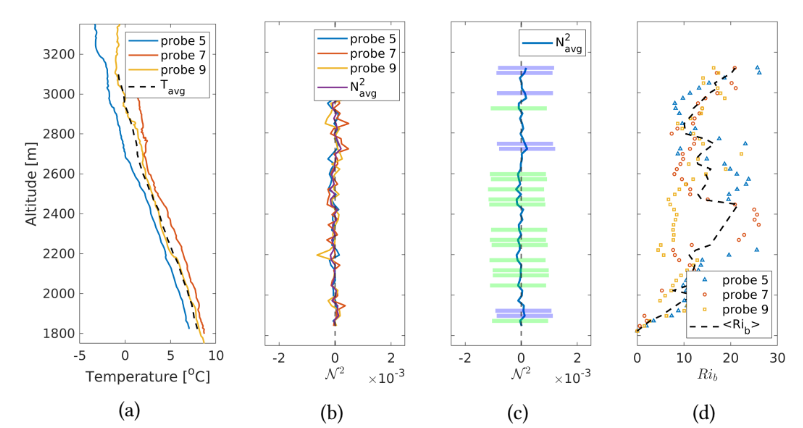
Figure 6: Temperature profile and Brunt-Väisälä frequency (OAVdA Experiment, November 3rd, 2022). (a) The vertical profile of temperature measurements throughout the altitude range. (b) The calculated Brunt-Väisälä frequency (N2 =gδT /T01/Δz ) as a function of altitude, where T0 = 281 K and g = 9.81 m/s2. (c) The average Brunt-Väisälä profile was calculated from the profiles of probes 5, 7, and 9. The shaded regions highlight the altitude ranges where all three probes exhibited a consistent temperature gradient: violet indicates a positive (stable) gradient, and green indicates a negative (unstable) gradient. (d) Estimated bulk Richardson number, Rib