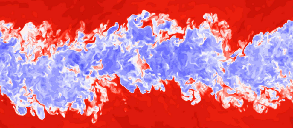
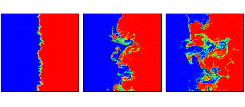
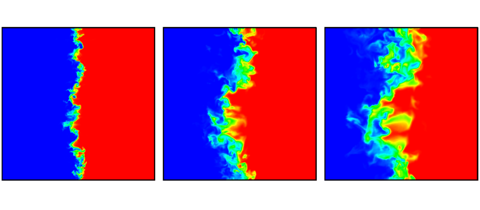
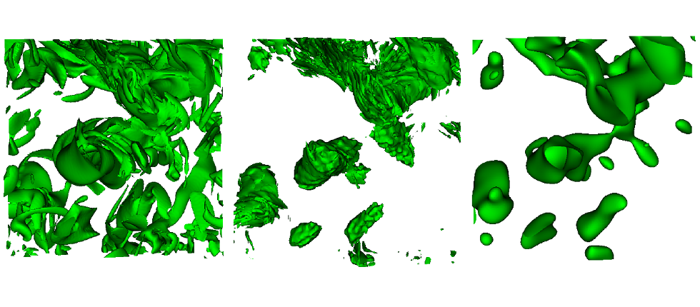
| | Diffusion of a passive scalar across the interface which separates two homogeneous and isotropic regions with different energy in 2D turbulence. The visualization shows the scalar field in the central part of the computational domain. The high turbulent energy velocity field is on the left of each image. The three different instants correspond, from left to right, to t/τ = 1, 5, 10, respectively. τ is the initial eddy turnover time of the high-energy region. (see Iovieno et al., J. Physics: Conf. Series 318, 2011)
|