27 Oct Gallery
Students Visualizations
Below is a brief description of each image. For further details, please visit the dedicated pages linked to each image.Visualization of a jet
This image captures the visualization of a jet flow using cigarette smoke. A desk lamp on the left side illuminates the smoke, highlighting the flow patterns and providing clear contrast to observe the jet’s movement and dynamics. (Photo: Giuseppe Pipia, 2015)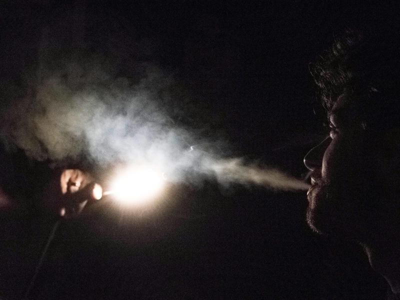
Flow visualization
Visualization of the flow produced by a cigarette. A desk lamp has been used to lighten the smoke. (Photo: Giuseppe Pipia, 2015)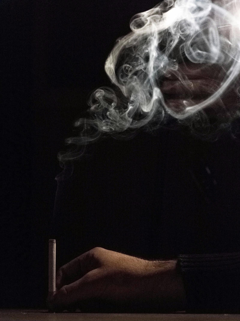
Poiseuille channel flow
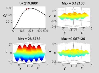
(Re=10000, k=5, Φ=π/2, antisymmetric initial condition). Perturbation velocity field in the physical plane (z, y) normal to the streamwise direction, x. See the MOVIE for the complete temporal evolution.
(Andrea Borio, Giuseppe Craparotta, Gloria Scaletta, Fluid Dynamics, Master Degree in Mathematical Engineering, 2012)

Poiseuille channel flow
(R=10000, k=0.9, symmetric initial condition, Φ=π/12). Perturbation velocity field in the physical plane (x, y) normal to the spanwise direction, z. See the MOVIE for the complete temporal evolution. (Alessandro Bay, Melania Carfagna, Anna Sapienza, Fluid Dynamics, Master Degree in Mathematical Engineering, 2012)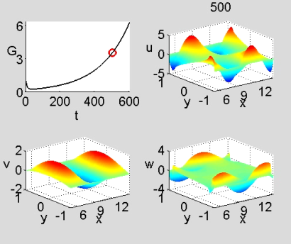
Homogeneous and isotropic turbulence
Pseudocolor plot for the dimensionless velocity component u, 256^3 grid. (Fabrizio Donati, 2011)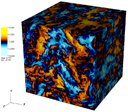
Homogeneous and isotropic turbulence
Isosurface plot of vorticity magnitude. Top: |ω| < 1 (left) and 1 <|ω| < 2 (right). Middle: 2 < |ω| < 3 (left) and 3 < |ω| < 4 (right). (Fabrizio Donati, 2011)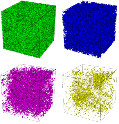
Homogeneous and isotropic turbulence
Velocity vector plot 0 ÷ 6 (cyan to black) on a vorticity magnitude pseudocolor plot 0 < |ω| < 4 (yellow to red) for different filtered fields. Top left: reference field. Top right: filament 0-150/50. Bottom left: cross 0-20. Bottom right: cross 30-150. (Fabrizio Donati, 2011)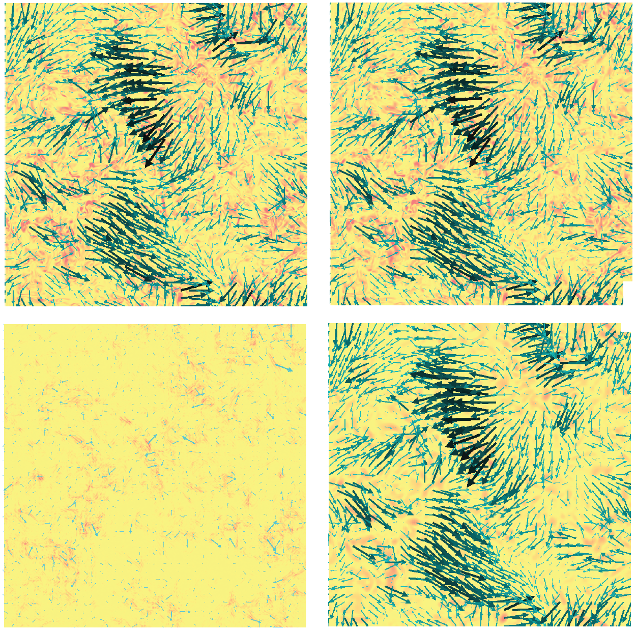
Turbulent channel flow
Direct numerical simulation, Re_τ=180. Streamwise velocity fluctuations at y+=21.6. (The mean flow is from left to right) (2010).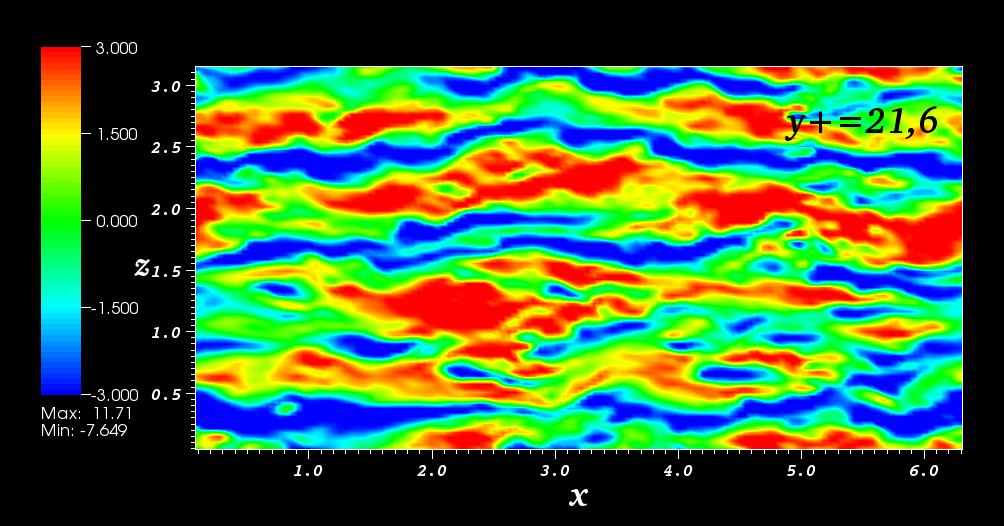
Turbulent channel flow
Direct numerical simulation, Re_τ=180. Streamwise velocity fluctuations at y+=180. (The mean flow is from left to right) (2010).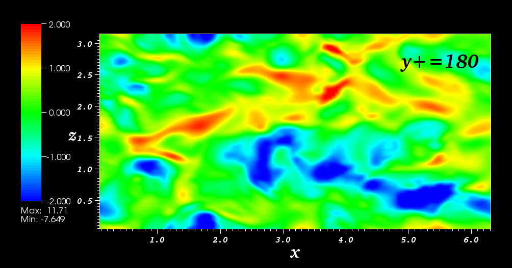
Hypersonic Jets
Astrophysical Jets: laboratory experiments
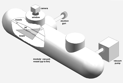
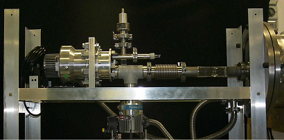
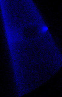
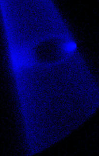
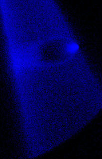
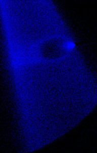
New Journal of Physics (2011): videoabstract The experimental setup. By means of a fast piston mounted on the left, the jet gas is compressed to stagnation pressures ranging from 0.1 to 0.7 MPa ,and is accelerated by a de Laval nozzle. The jet travels along a vessel filled with the desired ambient gas (at pressures in the 1.5–100 Pa range) and meets an electron sheet. The sheet ionizes the gases and makes a plane section of the flow visible; these images are acquired by an intensified high-speed CMOS camera.
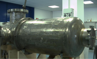
 The vessel
– Jet generation at the nozzle (movie).
 The electron gun
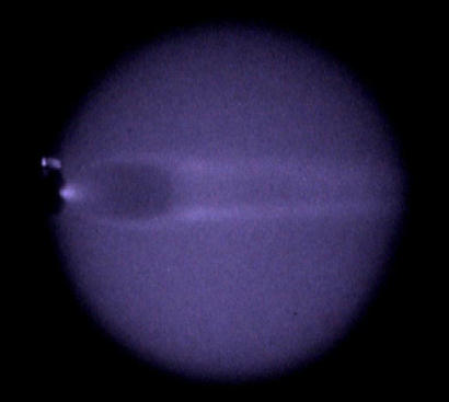
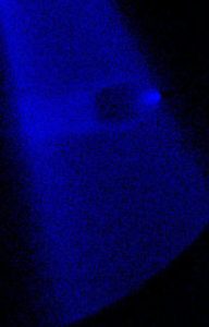
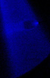
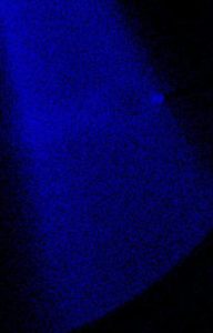
 Underexpanded jet, He/Ar (see movie)
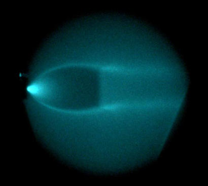
 Underexpanded jet, Ar/He
 Light jet, helium in xenon, M= 16.1. Density maps: numerical simulations and experimental measurements.
– Higher resolution picture
– movie (numerical simulation)
– movie (experiment)
 |
 |
 |
|
 |
 |
 |
|
 |
 |
 |
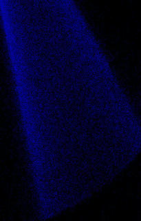
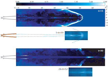 Heavy jet, Xenon in air, M= 15. Density maps: numerical simulations and experimental measurements.
– Higher resolution picture
– movie (numerical simulation)
– experimental movies (Xe in Ar): original and reworked by means of multicorrelation techniques.
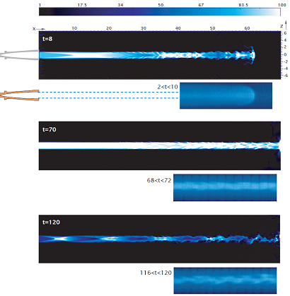 Light jet, numerical simulation.
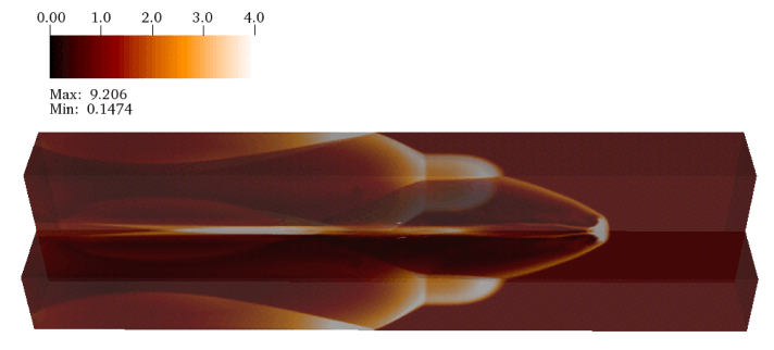
t = 15 t_jet

t = 20 t_jet

t = 30 t_jet

t = 40 t_jet

t = 50 t_jet

t = 60 t_jet
Large-eddy simulation of hypersonic jets Visualizations from a large-Eddy simulations of a compressible with M=5. The simulation follows the temporal evolution of a initially round 3D jet subject to periodicity conditions along the longitudinal direction. The smagorinsky model has been used together with the selective filtering procedure.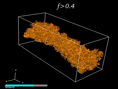 Large-eddy simulation of a hypersonic jet at M=5. The figure shows the underresolved regions where the small-scale indicator f is larger than the threshold 0.4.
For more details refer to CPC (2007) and (2013)
A complete movie of this time-evolving jet can be seen here.
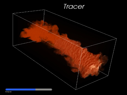 Large-eddy simulation of a hypersonic jet at M=5. The figure shows a passive tracer introduced at t=0 in the initially round jet. A complete movie of this time-evolving jet can be seen here.
For more details on the simulation refer to CPC (2007) and(2013)
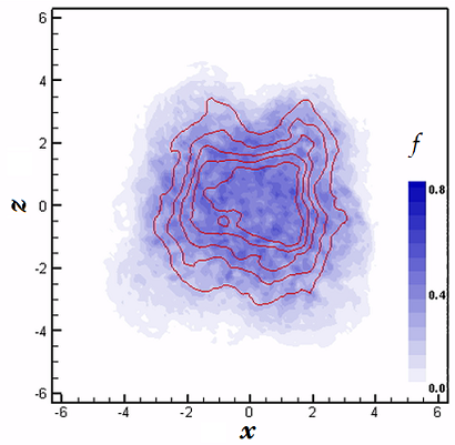 Large-eddy simulation of a hypersonic jet at M=5. The blue contours indicate the fraction of space where sub-filter scales are present, and the red lines are the isolines of the streamwise velocity u/u0.
See movie.
Turbulent Mixing
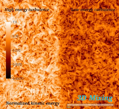 Shearless turbulent mixing. Visualization of the kinetic energy in the central part of the mixing in a plane (x, y1), (y2 = const). The higher energy region has a Taylor microscale Reynolds number equal to 150, the energy ratio is 6.7. For more details on the flow, see the paper in Physical Review Letters (2011).
The time evolution of the mixing layer can be seen in this movie, which shows the kinetic energy in the first 6 eddy turnover times.
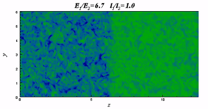 Shearless turbulent mixing. Visualization of the kinetic energy in a plane. The higher energy region has a Taylor microscale Reynolds number equal to 45.
– energy ratio 6.7, uniform integral scale (see movie)
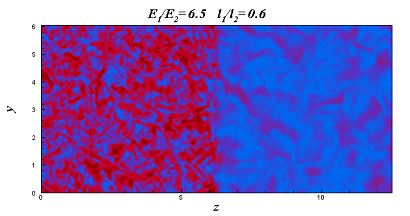 – as above, but the integral scale gradient is opposite to the kinetic energy gradient (see movie).
Both movies last about 9 eddy turnover times.
For more details on these simulations, refer to JFM (2006).
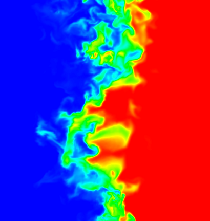 Passive scalar diffusion through a kinetic energy gradient. The higher energy turbulent region (Reλ=150) is on the left of the image, the lower energy region is on the right.
The time evolution of the scalar diffusion is shown by the following movies:
- Reλ=150 (6002x1200 simulation, colors as in the figure)
- Reλ=150 (6002x1200 simulation)
- Reλ=250 (10242x2048 simulation)
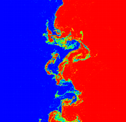 Passive scalar diffusion through a kinetic energy gradient in a two-dimensional flow. The higher energy turbulent region (Reλ=150) is on the left of the image, the lower energy region is on the right.
The time evolution of the scalar diffusion is shown by the following movies:
- 10242 simulation with hyperviscosity
- 2048×4096 NS simulation, Rel=3500.
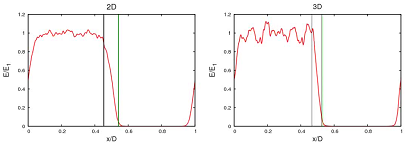 Kinetic energy profiles, comparison between the two-dimensional and the three-dimensional flow. The black vertical lines indicate the borders of the mixing layers, and the vertical green line indicates the position of maximum intermittency (see movie).
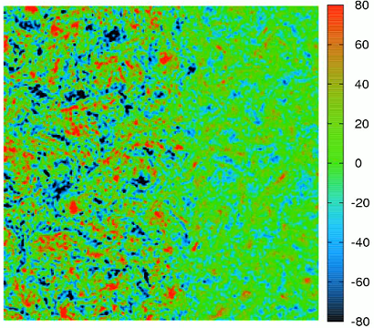 Vorticity field, two-dimensional simulation (see movie).
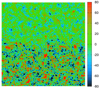 Vorticity field in the presence of a stable stratification (Fr=10), preliminary result from a two-dimensional simulation (see movie).
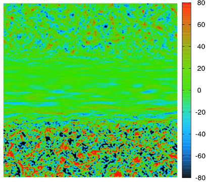 Vorticity field in the presence of a stable stratification (Fr=0.1), preliminary result from a two-dimensional simulation (see movie).
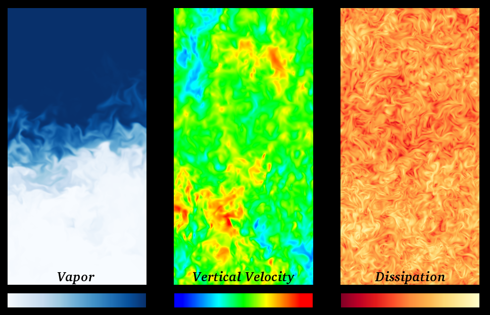 Diffusion of vapour through a horizontal interface in a stratified environment. The image shows a vertical plane (see also the movie).
For more details, see the proceedings of UIT-32.
Linear Wave Packets
Plane Poiseuille flow Figure 1. Localized wave packet in Plane Poiseuille flow with Re=1000. An impulsive initial condition, located at the channel mid-plane is obtained by linear superposition of 7380 waves. The longitudinal (α) and transversal (β) components of the polar wavenumber span the range [0,10] and [-10,10], respectively. The visualization represents the three components of the perturbation velocity after 60 time scales and at y=0.5. All the spatial coordinates are nondimensional (the reference length is the channel half thickness), and the basic flow is from left to right [movie U] [movie V] [movie W].
Blasius boundary-layer flow
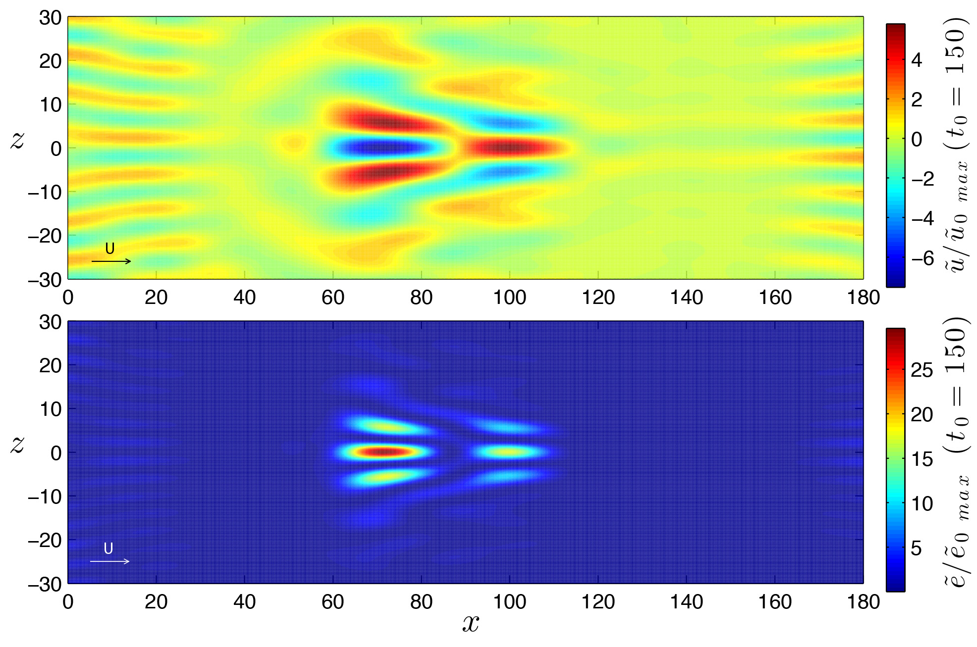 Figure 2. Localized wave packet in Blasius flow with Re=1000. An impulsive initial condition, located near the wall at (x,z)=(0,0) is obtained by linear superposition of 365 waves with polar wavenumber within the range [2.5± 3.8]. The visualization represents the longitudinal component of the perturbation velocity (top panel) and the perturbation kinetic energy (bottom panel) after 150 time scales and at y=0.5. All the spatial coordinates are nondimensional (the reference length is the displacement thickness δ*), and the basic flow is from left to right [movie U] [movie V] [movie W] [movie E]
Hydrodynamic Stability
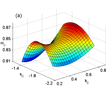
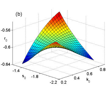 Figure 1. Bluff-body wake. Saddle points multidimensional map: (a) ω0(k0,s0) and (b) r0(k0,s0), Re=35, 4 diameters downstream the body.
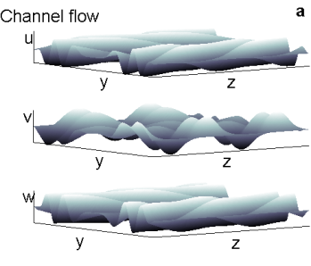
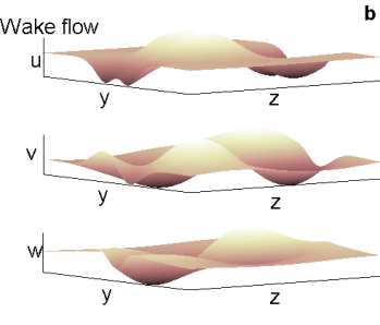 Figure 2. Snapshots of the perturbation velocity field in the physical plane (y, z) normal to the streamwise direction, x. (a) Channel flow: Re = 10000, t = 20, ϕ = 3/8 π, antisymmetric initial condition, k = 1.5. (b) Wake flow: Re = 100, wake section: 50 body lengths downstream, t = 45, ϕ = 3/8 π, antisymmetric initial condition, k = 0.7.
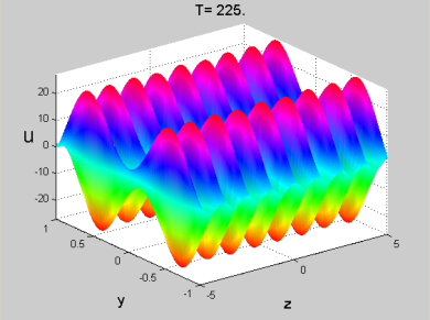 Figure 3. Longitudinal component of the perturbation velocity field in the physical plane (y, z) normal to the streamwise direction, x. Poiseuille channel flow: Re = 10000, t = 225, ϕ = π/2, antisymmetric initial condition, k = 5. See the MOVIE for the complete temporal evolution.
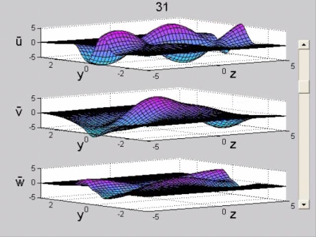 Figure 4. Amplified configuration. Wake flow (R=100, x_0=10, k=1.7, symmetric initial condition, Φ=π/8). Perturbation velocity field in the physical plane (y, z) normal to the streamwise direction, x. See the MOVIE for the complete temporal evolution.
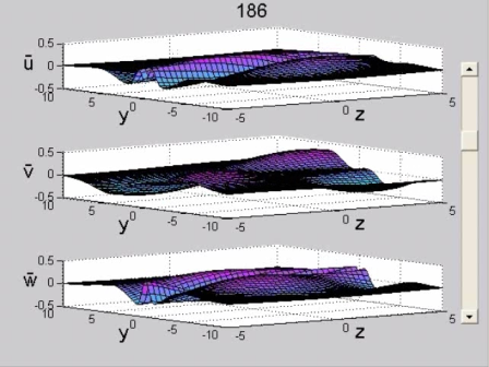 Figure 5. Weakly amplified configuration. Wake flow (R=100, x_0=10, k=0.6, asymmetric initial condition, Φ=π/4). Perturbation velocity field in the physical plane (y, z) normal to the streamwise direction, x. See the MOVIE for the complete temporal evolution.
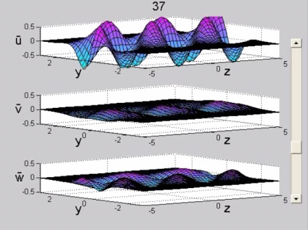 Figure 6. Damped configuration. Wake flow (R=100, x_0=10, k=1.7, symmetric initial condition, Φ=3/8π). Perturbation velocity field in the physical plane (y, z) normal to the streamwise direction, x. See the MOVIE for the complete temporal evolution.


