Intermittency acceleration of water droplet population at cloud edges (INDROPS)
Principle investigator: Prof. Daniela Tordella
Research Group: D. Tordella, Shahbozbek Abdunabiev, Ludovico Fossa, Mina Golshan, Chiara Geron
Collaborated with CINECA, with Dr. C. Cavazzoni
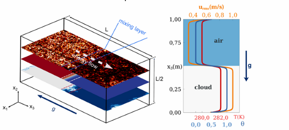
The project fundamentally focused on intermittency acceleration of water droplet populations inside the interface mixing region between warm clouds and the environmental clear air. The direct numerical simulations (DNSs) conducted in a 3D domain. the computational domain schematics is a given in Fig 1.
Figure 1. Schematics of the simulation domain (left panel) and of the initial profiles of the rms velocity (orange), temperature (red) and vapour content (blue) (right panel). The turbulent kinetic energy flow is from bottom to top along x3 direction, E1/E2= 10.
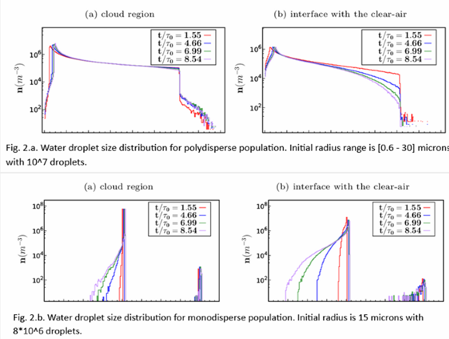
During our recent CINECA project (IsC72_RAINFALL), we have performed DNS simulations to analyse the temporal evolution of a small portion of the top of a cloud. In these simulations, the Eulerian description of the turbulent velocity, temperature, and vapor fields (see Fig. 1) is combined with the Lagrangian description of two different ensembles of cloud droplets, that is, with a monodisperse and a polydisperse size distribution (see Fig. 2. a,b).
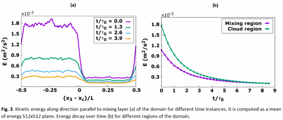
In this study, we have tried to be aligned with respect to the real warm cloud situation as much as possible. We have considered an observation duration of the order of a few seconds. During this time, the kinetic energy decays throughout the system by 95%(see Fig. 3 . b). It should be recalled that the kinetic energy inside the interfacial layer (the shear-free turbulent mixing layer that matches the cloud and clear air regions) also decays spatially by nearly 85%.
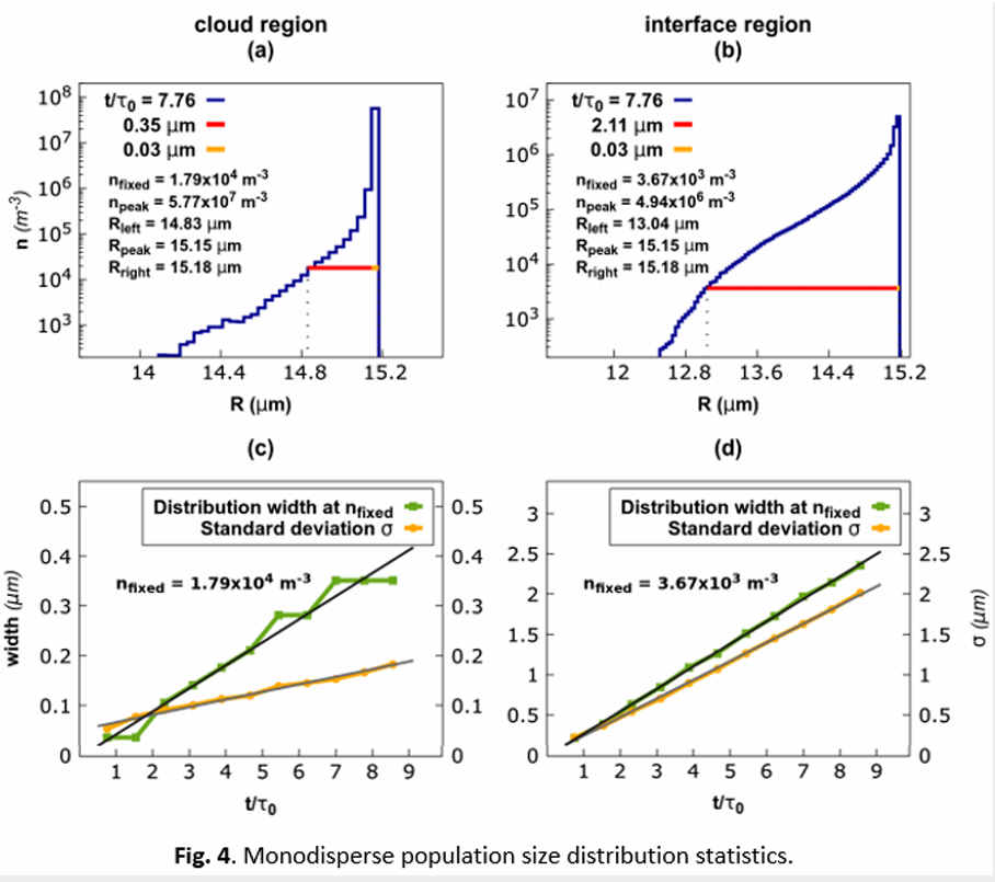
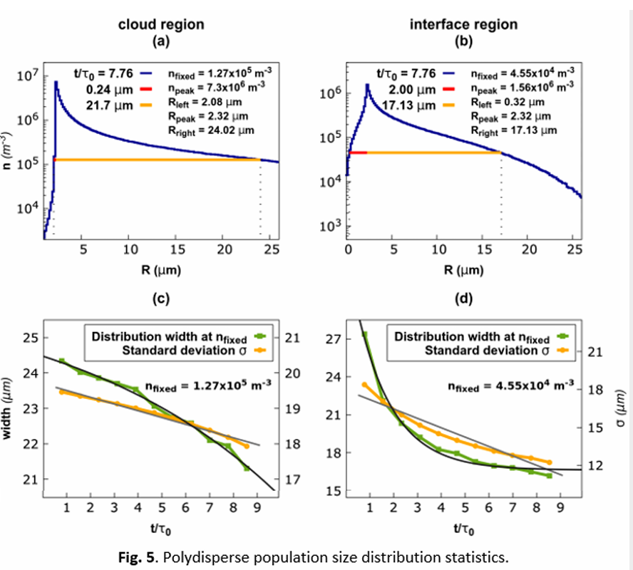
We observed, with respect to the cloud region, in the interfacial layer, both the monodisperse (see Fig. 4) and poly-disperse (see Fig. 5) populations evolve at least 5 times faster. This acceleration of the dynamics is remarkable and is somewhat counterintuitive.
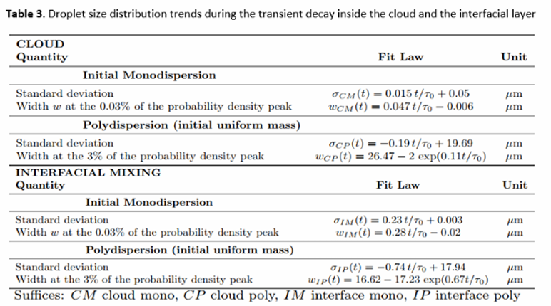
Better comparison of dynamic acceleration in cloud and interfacial layer can be done by looking fit functions (trends). The fit functions for standard deviation and width (at the fixed droplet concentration) of the size distribution are obtained for both regions and size populations, see the following Table 3.
We used linear and exponential fit functions (of t/τ0) for the standard deviation and width of the size distribution, respectively. When we look at the linear fit of standard deviation for cloud and mixing regions, we can see fit functions for the mixing have a higher slope than the cloud ones for both monodisperse and polydisperse populations. So, the rate of population evolution is much faster in the interfacial mixing region than in the cloud region. Furthermore, the polydisperse size distribution is shrinking (slope < 0) over time, while the monodisperse one is widening (slope > 0). We can estimate how long it can take to have the same standard deviation of two size distributions. Based on our estimation, it takes ~20 t/τ0 (eddy turnovers) in the mixing and ~100 t/τ0 in the cloud. But we run our simulations only for ~10 eddy turnovers, and kinetic energy is decaying fast enough. In order to validate our fit functions, we need to watch the evolution of the droplet population in longer simulation runs.
We computed droplet response times with the above formula for the polydisperse population([0.6-30] micron). Our integration time step was 3.8e-4 seconds, which is not sufficient to consistently resolve the response time of small particles inside the population. So, we have to use a smaller time step in the following simulations.